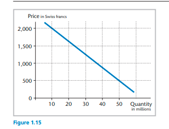
dolution

dolution.

Developing and altering organizational charts is an important skill for strategists to possess. This exercise can improve your skill in altering an organization’s hierarchical structure in response to new strategies being formed. Instructions Step 1 Develop an organizational chart for Nestlé. On a separate sheet of paper, answer the following questions: • What type of organizational chart have you illustrated for Nestlé? • What improvements would you recommend for the Nestlé organizational chart? Give your reasoning for each suggestion. Step 2 Now consider the following: • What aspects of your Nestlé chart do you especially like? • What type of organizational chart do you believe would best suit Nestlé? Why?

dolution

 
"Looking for a Similar Assignment? Get Expert Help at an Amazing Discount!"

dolution

dolution.

The Return to Education and the Gender Gap

In addition to its intellectual? pleasures, education has economic rewards. As the boxes in Chapters 3 and 5? show, workers with more education tend to earn more than their counterparts with less education. The analysis in those boxes was? incomplete, however, for at least three reasons.? First, it failed to control for other determinants of earnings that might be correlated with educational? achievement, so the OLS estimator of the coefficient on education could have omitted variable bias.? Second, the functional form used in Chapter

5long dash—a

simple linear

relationlong dash—implies

that earnings change by a constant dollar amount for each additional year of? education, whereas one might suspect that the dollar change in earnings is actually larger at higher levels of education.? Third, the box in Chapter 5 ignores the gender differences in earnings highlighted in the box in Chapter 3.

All these limitations can be addressed by a multiple regression analysis that controls for determinants of earnings? that, if?omitted, could cause omitted variable bias and that uses a nonlinear functional form relating education and earnings. The Return to Education and the Gender Gap table summarizes regressions estimated using data on? full-time workers, ages 30 through? 64, from the Current Population Survey? (the CPS data are described in Appendix? 3.1). The dependent variable is the logarithm of hourly?earnings, so another year of education is associated with a constant percentage increase? (not dollar? increase) in earnings.

The Return to Education and the Gender Gap table has four salient results.? First, the omission of gender in regression? (1) does not result in substantial omitted variable? bias: Even though gender enters regression? (2) significantly and with a large?coefficient, gender and years of education are? uncorrelated; that?is, on average men and women have nearly the same levels of education.?Second, the returns to education are economically and statistically significantly different for men and? women: In regression? (3), the

t?-statistic

testing the hypothesis that they are the same is 7.02.? Third, regression? (4) controls for the region of the country in which the individual? lives, thereby addressing potential omitted variable bias that might arise if years of education differ systematically by region. Controlling for region makes a small difference to the estimated coefficients on the education? terms, relative to those reported in regression? (3). Fourth, regression? (4) controls for the potential experience of the? worker, as measured by years since completion of schooling. The estimated coefficients imply a declining marginal value for each year of potential experience.

The estimated economic return to education in regression? (4) is? 10.32% for each year of education for men and? 11.66% for women. Because the regression functions for men and women have different? slopes, the gender gap depends on the years of education. For 12 years of? education, the gender gap is estimated to be? 29.0%; for 16 years of? education, the gender gap is less in percentage? terms, 23.7%.

These estimates of the return to education and the gender gap still have? limitations, including the possibility of other omitted?variables, notably the native ability of the? worker, and potential problems associated with the way variables are measured in the CPS.? Nevertheless, the estimates in the Return to Education and the Gender Gap table are consistent with those obtained by economists who carefully address these limitations. A survey by the econometrician David Card? (1999) of dozens of empirical studies concludes that labor? economists’ best estimates of the return to education generally fall between? 8% and? 11%, and that the return depends on the quality of the education. If you are interested in learning more about the economic return to? education, see Card?(1999).

Read the box “The Return to Education and the Gender Gap.” The Return to Education and the Gender Gap Dependent variable: logarithm of Hourly Earnings. Regressor Years of education 0.1001* (0.0011) -0.432** (0.024) 0.0121* (0.0017) 0.1051 (0.0012) 0.1035* (0.0009) 0.1050 (0.0009) – 0.263** (0.004) Female 0.451* (0.024) 0.0134 (0.0017) 0.0149** (0.0012) – 0.000203** (0.000027) 0.095** (0.006) 0.092 (0.006) -0.021* (0.007) Female x Years of education Potential experience Potential experience Midwest South West
1.533 (0.012) 0.208 Intercept 1.629 (0.012) 0.258 1.697* (0.016) 0.258 1.433 (0.023) 0.267 The sample size is 52,970 observations for each regression. Female is an indicator variable that equals 1 for women and 0 for men. Midwest, South, and Wost are indicator variables denoting the region of the United States in which the worker lives: For example, Midwest equals 1 if the worker lives in the Midwest and equals 0 otherwise (the omitted region is Northoast). Standard errors are reported in parentheses below the estimated coefficients. Individual coefficients are statistically significant at the +5% or 1% significance level. Scenario A Consider a man with 14 years of education and 5 years of experience who is from a western state. Use the results from column (4) of the table and the method in Key Concept 81 to estimate the expected change in the logarithm of average hourly earnings (AHE) associated with an additional year of experience. The expected change in the logarithm of average hourly earnings (AHE) associated with an additional year of experience is%. (Round your response to two decimal places.)
The Expected Effect on Y of a Change in X4 in the Nonlinear Regression Model The expected change in Y. ??, associated with the change in X1, ???, holding X2, , Xk constant, is the difference between the value of the population regression function before and after changing X1, holding X2,, XK constant. That is, the expected change in Yis the difference The estimator of this unknown population difference is the difference between the predicted values for these two cases. Let fX,. X2. Xk) be the predicted value of Y based on the estimator fof the population regression function. Then the predicted change in Yis 12k 12 k

dolution

 
"Looking for a Similar Assignment? Get Expert Help at an Amazing Discount!"

dolution

dolution.

Crash Tests The Insurance Institute for Highway Safety regularly tests cars for various safety factors. In one such test, the institute tests the bumpers in 5-mile per hour (mph) crashes. The following data represent the cost of repairs (in dollars) after four different 5-mph crashes on small utility vehicles. The institute blocks by location of crash, and the treatment is car model.

(a) Normal probability plots for each treatment indicate that the requirement of normality is satisfied. Verify that the requirement of equal population variances for each treatment is satisfied. (b) Is there sufficient evidence that the mean cost of repairs is different among the four SUVs at the  level of significance?

(c) If the null hypothesis from part (b) was rejected, use Tukey’s test to determine which pairwise means differ using a familywise error rate of .

dolution

 
"Looking for a Similar Assignment? Get Expert Help at an Amazing Discount!"

dolution

dolution.

Open the Trust data-set

a. Consider the allocation of respondents according to their job status (q54)

b. Using MDA, explore the role of the following predictors in explaining classification: age (q51), household size (q56), financial condition of the household (q61)

c. According to ANOVA tests, which predictors are statistically different across groups? Which predictor has the highest discriminatory power?

d. Which discriminant functions are significant according to the Chi-square test?

e. How much of the total variance does the first discriminant function explain?

f. Considering the structure matrix, try and label the discriminant functions

g. Compute the percentage of correctly predicted cases. Does allocation of all units to the modal category generate a better or worse prediction rate?

dolution

 
"Looking for a Similar Assignment? Get Expert Help at an Amazing Discount!"